Classification

The idea behind classification is a supervised learning methodology. So we’ll have a test and a training set. We also need to have a plotting platform to show the decision boundaries. ISLR, the book respected in this line of studies adequately discussed most of the problems. However, you can’t find the code for their charts easily.

If you sniff around the web, you’ll probably see how those plots are created. Combining that knowledge I had a crack at it.

Let’s go for a small dataset, Flea dataset. I don’t even want to discuss the variables!

We have two categories of fleas, so it’s a binomial, rather than a multinomial case. That’s convenient for us since we can use glm. I’ll be using a test and a training dataset to cross-validate our methods properly.

flea$type<-as.factor(flea$type)
rand<-sample(1:nrow(flea),5)
test<-flea[rand,]
train<-flea[-rand,]

A sample of 5 would suffice.

Also, let’s look at principal components of our explanatory variables to visualize our data.

require(ggbiplot)
PC_S<-princomp(flea[,2:5])
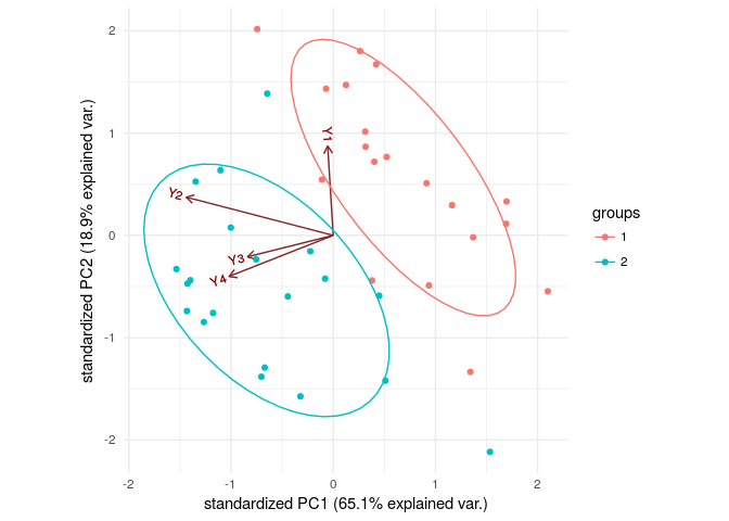
g<-ggbiplot(PC_S,groups = flea[,1],ellipse = TRUE,
            var.axes = TRUE)
g+theme_minimal()

detach(package:ggbiplot)

Ggbiplot is a package to visualize the data, aside from its use in dimension reduction by using principal components. It shows data points on a plane made by two most important principal components. We can distinct between these two groups by just looking at the plot. But how would we find it by math!

If you have any problems in installing ggbiplot, you should use the devtools package to install it from it’s GitHub repository.

install.packages("devtools")
require(devtools)
install_github("vqv/ggbiplot")

Let’s use logistics regression to classify now. Basically what we’ll do here is calculate odds for each point of being in one of our groups to being in the other based on logit link function (linear assumption on the relationship between the log odds of the response and explanatory variables).

Doing logistics regression will allow us to select the best model based on training dataset only. I have written a logistics model selection function, which will exhaustively look for the best model up to first degree interactions. We should never use this though for a larger set of variables since the possible models grow very fast.. $O(2^{\frac{p(p+1)}{2}})$

logistic_binomial_model_selection<-function(data,response){
  lis<-search()
  lis<-"package:plyr" %in% lis
  if (lis){detach(package:plyr)}
  require(knitr)
  require(dplyr)
  models<-function(var_names){
    var_names<-names(data[,-response])
    model_vars<-1
    for (j in 1:length(var_names)){
      mt<-combn(var_names,j)
      for (i in 1:ncol(mt)){
        if (j==2 & i==1){
          for (s in 1:ncol(mt)){
            cols<-combn(1:ncol(mt),s)
            for (w in 1:ncol(cols)){
              mt_int<-mt[,cols[,w]]
              inter<-unique(c(mt_int))
              if (s>1){
                tmp1<-apply(mt_int,2,paste,collapse=":")
                tmp1<-paste(c(tmp1,inter),collapse="+")
              }
              else {
                tmp1<-paste(mt_int,collapse = ":")
                tmp1<-paste(c(tmp1,inter),collapse="+")
              }
              other<-setdiff(var_names,inter)
              if (length(other)>0){
                for (k in 1:length(other)){
                  mt1<-combn(other,k)
                  for (l in 1:ncol(mt1)){
                    interact<-paste(c(tmp1,mt1[,l]),collapse = "+")
                    model_vars<-c(model_vars,interact)
                  }
                }
              }
              else {
                interact<-tmp1
                model_vars<-c(model_vars,interact)
              }
            }
          }
        }

        tmp<-paste(mt[,i],collapse="+")
        model_vars<-c(model_vars,tmp)
      }
    }
    return(model_vars)
  }

  models<-models(name)
  res<-data.frame(model="",Deviance=1,df=1)
  for (i in 1:length(models)){
    model<-eval(parse(text=paste("glm(data=data,",names(data)[response[1]],"~",
                                 models[i],",family=binomial('logit'))")))
    if(model$converged==TRUE){
      tmp<-data.frame(model=models[i],Deviance=model$deviance,df=model$df.residual)
      res<-rbind.data.frame(res,tmp)
    }
  }

  res<-res[-1,]
  res<-res%>%arrange(desc(df),desc(Deviance))

  res$df<-as.factor(res$df)
  best<-res%>%select(df,Deviance,model)%>%group_by(df)%>%summarize(Deviance=min(Deviance))
  best_models<-best%>%left_join(res)
  test<-rep(1,nrow(best_models))
  for (i in 1:(nrow(best_models)-1)){
    tb<-best_models%>%mutate_all(as.numeric)
    if (tb$Deviance[i]>tb$Deviance[i+1]){test[i]<-1}
    else {test[i]<-1-pchisq(tb$Deviance[i+1]-tb$Deviance[i],df=tb$df[i+1]-tb$df[i])}
  }
  best_models$GoodnessOfFit_test<-test
  best_models<-best_models%>%mutate(significance=ifelse(GoodnessOfFit_test<.05,"*",""))
  kable(best_models)
}

logistic_binomial_model_selection(data=train,response=1)

df	Deviance	model	GoodnessOfFit_test	significance
29	6.122172	Y1:Y3+Y1+Y3+Y4	0.6005315
30	6.396367	Y1+Y3+Y4	0.0708480
31	9.659630	Y1+Y2	0.0001287	*
32	24.320626	Y3	0.0000018	*
33	47.134008	1	1.0000000

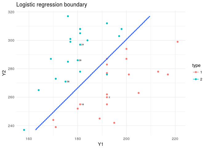
The best model here, shows we need only two variables. Y1 and Y2. So we wouldn’t have any plotting issues! If there were more than two, then we would have required mapping our boundary on several plots, consisting of plains made by such variables or we could have done it on the first 2 PCs.

model<-glm(data=train,type~Y1+Y2,family=binomial("logit"))

X_range<-seq(min(flea$Y1),max(flea$Y1),length.out = 300)
Y_range<-seq(min(flea$Y2),max(flea$Y2),length.out = 300)
XY_grid<-expand.grid(X_range,Y_range)
XY_grid<-tbl_df(XY_grid)
names(XY_grid)<-c("Y1","Y2")
XY_grid$pred_glm<-predict(model,XY_grid,type="response")
XY_grid$type<-ifelse(XY_grid$pred_glm<.5,1,2)
flea$index<-1:nrow(flea)

plt<-ggplot(data=flea,aes(x=Y1,y=Y2,col=type))+
  geom_point()+theme_minimal()+
  geom_text(data=flea[rand,],aes(x=Y1,y=Y2,label=index),nudge_x = 1,col="black",cex=2)
  plt+stat_contour(data=XY_grid,aes(x=Y1,y=Y2,z=type))+
  labs(title="Logistic regression boundary")

To see how our classifier worked we can check the misclassification error rates for the test data set and also the fit to the training dataset.

glm_prob<-predict(model,newdata = test[,-1],type = "response")
glm_pred<-ifelse(glm_prob<.5,1,2)
table(test$type,glm_pred)

##    glm_pred
##     1 2
##   1 3 0
##   2 0 2

cat("Misclassification error rate is:",percent(mean(glm_pred!=test$type)))

## Misclassification error rate is: 0%

glm_prob<-predict(model,newdata = train[,-1],type = "response")
glm_pred<-ifelse(glm_prob<.5,1,2)
table(train$type,glm_pred)

##    glm_pred
##      1  2
##   1 16  0
##   2  1 17

cat("Misclassification error rate (for train set) is:",percent(mean(glm_pred!=train$type)))

## Misclassification error rate (for train set) is: 2.94%

The compiled version of this document can also be found on Rpubs. Link to Document.